Welcome back to our series where we are sharing a step by step walkthrough of our data stack development process. In the previous iteration of this series we walked through how to initialize your selected Data Warehouse and connect it with your live data source(s) using an AirByte pipeline. If you have not read this or have not already set up your Data Warehouse and raw data pipeline, we highly recommend checking that out here before diving into data structuring and transformations.
In this post we will be discussing the Transformation portion of an ETL data stack — focusing on the deployment of Data Build Tool (dbt) to validate, clean, and organize raw data into production quality datasets. As we covered in Part 1 of our series, dbt is a widely compatible data transformation tool that provides a framework for structuring transformation workflows — allowing users to write modular SQL scripts that follow a defined build dependency order. These automated workflows ensure that transformations are validated and deployed consistently, with detailed lineage tracking that provides transparency into how datasets are created and interrelated.
Put simply, dbt operates on top of your data warehouse, allowing you create new tables or views in your database by running SQL queries on your raw data.
With built-in features like automated testing, version control integration, and documentation generation, dbt enables reliable, transparent, and organized data pipelines. We will dive into how to properly structure your project to ensure you benefit from scalability and operational efficiency offered by dbt as your business grows and data needs evolve. Just as with planning your data stack, it’s essential to start with a clear vision of your analytical goals and end-user needs. A well-defined ‘road map’ ensures effective data transformation and delivery for your stakeholders.
Configuring your dbt Environment
To get started with dbt, create your free account on www.getdbt.com. This needs to be done regardless of what method of implementation you have chosen for dbt, but we will be covering development via dbt Cloud. Once you have confirmed your account, you will be prompted to connect to your data warehouse(s) and a GitHub repository. In the event you run into an issue, dbt provides live documentation to direct you to finding the correct account information and desired authentication for your warehouse and version control account. These steps are rather straightforward but crucial since this sets your project repository, and this development connection to your warehouse will be the database engine that runs your project — dictating the SQL dialect you will need to use. It is also important to use the account you had pre-designated in Snowflake (or your other warehouse of choice) for dbt’s compute resources as this will make tracking expenses and performance easier for your live pipeline. The Production environment we will create later for our deployment job will be based on this connection, so ensure that it is configured to utilize the resources you set aside for it.
Once initialized, dbt sets up your project with a basic folder structure that is ready for development. Unlike relational databases that organize data through tables and keys, a dbt project relies on files, folders, and consistent naming conventions. To ensure effective data transformation, your project’s structure must be clear and purposeful — guiding how transformations are grouped and directed. The goal is to transform source-conformed data into business-conformed data that is tailored to the needs of your business and its end users.
A dbt project has three key components: the Directed Acyclic Graph (DAG), the folder and file structure, and the output to the warehouse. Building a clear chain of models simplifies troubleshooting by isolating errors to specific operations — avoiding the confusion of a single block of faulty SQL code.
The DAG visualization in dbt Cloud ensures your pipeline flows logically, resembling an arrow or funnel leading to the final output. To streamline transformations, we recommend organizing models into three levels: staging, intermediate, and marts/entities. This structure compartmentalizes steps, helps catch errors quickly during development, and optimizes resource use in production.
Two fundamental principles of software development also apply to creating your dbt pipeline: DRY (Don’t Repeat Yourself) and KISS (Keep It Simple, Stupid). These principles remind us to maintain simplicity and minimize repetition throughout the process.
Staging your Pipeline
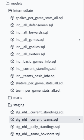
Now that you are set up in your IDE and dbt has generated a blank project, we can begin defining our project. As when constructing almost any project, laying a solid foundation is critical to the integrity of the entire system. Begin by familiarizing yourself with the default project structure before modifying your model folders to match the desired, layered structure as seen in the below example.

Before writing SQL models, you must configure the YAML files that define your project’s structure. The primary file, dbt_project.yml, serves as your project’s blueprint — managing configurations for directories (e.g., tests, macros, metrics, models) and project settings. While the default template generated by dbt is often sufficient in many respects, we recommend focusing on defining your models directory, paths, materialization settings, and tests in the bottom section — ensuring they align exactly with your folder structure and YAML conventions. Additionally, you can define individual models with descriptions, materialization settings, sub-schema designations, and simple tests (e.g., unique or not null quantifiers) for more detailed control. Misalignment can result in errors so it’s worth taking the time to do this right!

With the initial YAML configuration complete, the next step is defining your sources in the sources.yml file. This file organizes data sources by specifying each source and its corresponding datasets. Using YAML syntax, define each source with a pseudonym representing the combination of warehouse and internal schema to extract from. For each source, list the tables along with their names, descriptions, and any relevant variables. Clear and descriptive naming is crucial for easier identification and development, as these tables will be accessed later using the dbt format {{ source('source_name', 'table_name') }}.
In projects with multiple data sources, it’s best to create subdirectories within the staging folder for each source and include a separate
sources.ymlfile in each subdirectory. This approach helps keep your staging layer well-organized and easier to manage.

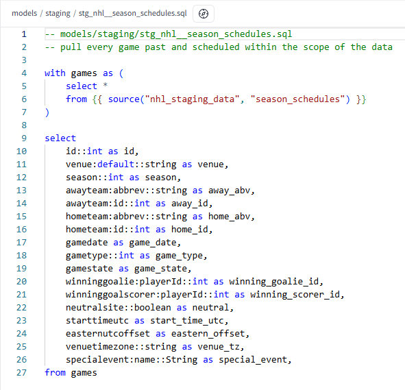
With the YAML configuration complete, you can begin writing and chaining models for your pipeline. It’s important to note that a dbt model is essentially a SQL file that runs the select query within it—if the file contains no queries or multiple queries, it will fail to run. That said, within each file you can include as many CTEs and as much functionality or complexity as your SQL engine supports. For those new to dbt, it’s best to start with simple models, like the example below, and gradually add complexity. This approach helps you become familiar with dbt’s syntax and concepts while building confidence in your pipeline development.

As you develop more models at all levels, file naming is critical and having a convention will make working with your models infinitely easier since models are monikered based on the file name. For example, having a base.sql model in each of your staging, intermediate, and marts folders will create three identically named models and lead to devastating errors. Thus, having a unique name that concisely adds the path and a descriptive name, such as stg__base (or stg_stripe__clients for multi-source projects), is a much better practice. Following this convention witll make navigating and debugging your project much more simple in the future!
To reference a model in dbt, we use the
{{ ref('model_name') }}syntax to query that model, which highlights the need for a clear naming convention

Writing Models in the Staging Layer
At the risk of being redundant it is worth emphasizing once more that maintaining a clear project structure and consistent compartmentalization is crucial. In the staging layer, focus on creating small, consistent, atomic building blocks — each originating from its source and easily integrated with others. These models should primarily handle simple tasks like importing raw data, typecasting fields, and validating data. For example, with client data, ensure identifier fields have the correct data types and maintain consistent formats for dates and strings. This foundational work avoids redundancies in downstream transformations. Avoid applying complex transformations at this stage, as it can overcomplicate the project, waste resources, and lead to unnecessary repetition. Instead, ensure the source data is clean, validated, and ready for downstream modeling.

In our NHL project, even the most complex staging model (see above) only performs basic tasks like type casting, re-aliasing, and extracting JSON fields. Importantly, it avoids substantial manipulation — aligning with the purpose of the staging layer. This example also highlights a key concept in dbt models (and in complex SQL code in general): the Common Table Expression (CTE). CTEs act as virtual tables created at query execution, helping to save resources by avoiding the materialization of intermediate steps. They also improve code readability, organization, and debugging.
To align with best practices, source invocations should always be placed inside CTEs. This approach separates the source connection from transformations – enabling incremental development and easier testing. For the staging model above, wrapping transformations in a CTE before the final query execution would further enhance structure and maintainability
It is important to note here, that if you are developing in dbt Cloud and attempt to reference a model not yet built, it will fail. So, when creating your models, ensure that you use the command line at the bottom of the IDE to run your models as you go — these models will be used exclusively in the staging environment we created earlier and dbt will automatically create a schema in your warehouse dedicated to housing these models. As we build more complex models and continue to update them, it is critical that you run your models in your staging environment consistently to propagate any development changes down stream.

Transforming your Data
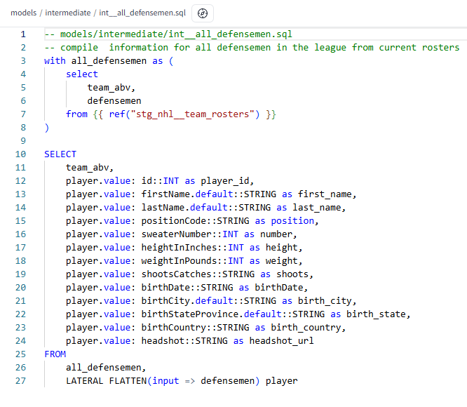
Now that we have our raw data cleaned, standardized, and loaded into models, we can begin the bulk of our transformations. Keeping in mind our layering of transformations, the intermediate layer serves to simplify our source data, re-grain models, and isolate complex operations. Here we want to implement any complex, reusable transformations or aggregations. For example if we have client data from multiple sources, creating an intermediate model that joins the client data from these sources will prove useful for later models. In our project, we had individual game data for players, which we re-grained to the season level and performed aggregations for players and teams is the backbone of our analytical tables. The example below exemplifies this by un-nesting a semi-structured column in a flat model to be used for all future player related models.

The intermediate layer also serves as the perfect place to perform unique operations that have specific criteria and heuristics beyond simple aggregation. Isolating these specialized processes simplifies debugging and optimization by allowing you to trace issues or gaps back to specific models. As you can imagine, compiling a full set of transformations into one massive select query will get ugly quickly. As a result, how you develop these intermediate models is crucial to collaborative development. Breaking specific transformations into isolated CTEs within your model (as seen below) is a great way to create clean and readable code that can be easily expounded upon.
Keep in mind that your data warehouse determines the data types, functions, and transformations you can use. You’ll need to adhere to the syntax and limitations of its specific SQL dialect.
Before reaching the marts layer and building output tables, our DAG should ideally resemble a funnel pointing to the right. As we transition from source-conformed to business-conformed data, we combine narrow, isolated tables into broader, richer business concepts. This structure creates a cohesive and flexible set of components that can be easily configured to address diverse business questions and meet specific data needs.

Finalizing your Data
Finally we arrive at the last transformation layer, known as the marts or entity layer, where models are designed for end-user consumption. Each model in this layer should represent a distinct business entity or analytical concept – containing all relevant data for that entity at a granular level. These models should be as comprehensive as possible for their specific ‘object’ without aggregating data across other marts. For instance, client, payment, and invoice marts should remain distinct, while in our NHL example, team marts cover information, rosters, and statistics, and player marts handle similar categories for players. Any further aggregation (e.g., player stats over time) belongs in the intermediate layer or becomes a metric.
Think of marts as summaries of business entities — reinforcing the upstream project structure and culminating in materialized entity tables for end users. Simple, clear naming conventions, such as ‘rosters,’ ‘standings,’ or ‘team_stats,’ help ensure models are easily identifiable. If you find yourself combining data from more than three upstream models, consider moving some transformations to the intermediate layer.
The purpose of this layer is to tailor the data to match the needs of dashboards, machine learning models, apps, or other use cases. It’s crucial to ensure outputs are well-organized and named — with models not intended for broad use either omitted from materialization or isolated in dedicated areas. This approach ensures clarity, efficiency, and alignment with business needs.
Creating and Deploying the Job
Once you’re confident your project runs smoothly in the staging environment, it’s time to configure your deployment job. In the Deploy tab, start by creating a production environment. This involves selecting the desired warehouse connection, designating it as a ‘Production’ environment, and giving it a descriptive name. Note that this environment will create a PROD schema in your warehouse if it doesn’t already exist.
Next, set up a deploy job by selecting your production environment and configuring the job’s execution timing and settings. When scheduling the job, ensure it aligns with your source data updates so the dbt job always runs on fresh data. You can also customize how the dbt build command is executed. Options include generating documentation, checking source freshness, or running a series of specific dbt commands tailored to your needs instead of a standard dbt build invocation. This flexibility allows you to optimize your deployment for your project’s unique requirements.

A Quick Aside on Useful dbt Commands
dbt commands are the backbone of working with dbt projects, enabling users to develop, test, and deploy their models effectively. When working with dbt Cloud, these are invoked in the IDE’s command line for development and testing, or as list of commands in the specifications of a deployment job.
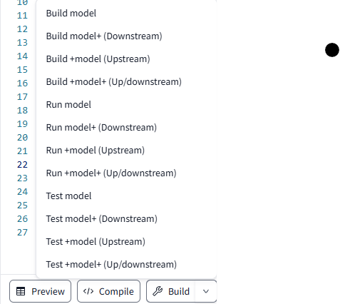
Two of the most important commands aredbt run, which compiles and executes models to generate tables in your database and dbt build, a comprehensive command that runs, tests, and seeds your project in one step. The dbt test command ensures data integrity by validating assumptions and detecting anomalies, while dbt debug helps troubleshoot connectivity issues. Additionally, you can generate interactive project documentation to give you a visual overview of your data pipeline with dbt docs generateor by checking the associated execution setting for a job, as seen above. Finally, while developing individual models, you can choose from the dropdown of available, pre-formatted commands, as seen below, to run on your development environment for that given model.

Conclusion
In summary, building an effective dbt pipeline requires careful planning and adherence to best practices at each layer — from staging to intermediate and finally to marts. By focusing on clarity, modularity, and alignment with business needs, your project can deliver reliable, scalable, and actionable insights. Whether you’re just starting out or refining an existing pipeline, following these principles ensures your data workflows remain efficient and adaptable as your organization grows. As always, if you have any questions or thoughts please drop a comment below or reach out to us at info@southshore.LLC
